Machine Learning

Flow-Like turns classical machine learning into an inspectable flow: prepare the data, fit the model, measure it, save it, and replay the same contract at prediction time. The important choices stay visible as nodes instead of disappearing inside a notebook.

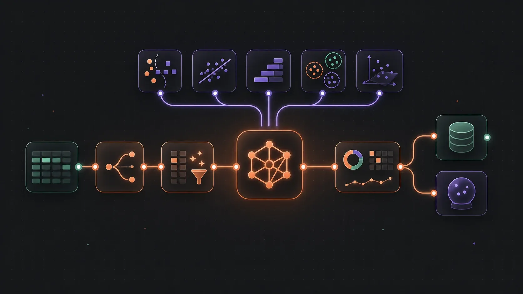
A label-free Flow-Like machine-learning system connecting tabular data, splitting and preprocessing to a central model, task families, evaluation, model storage, and predictions

Browse the Machine Learning node catalog for the complete pin schemas and defaults of every node named here.

Choose the learning task

Start with the target column, not the algorithm.

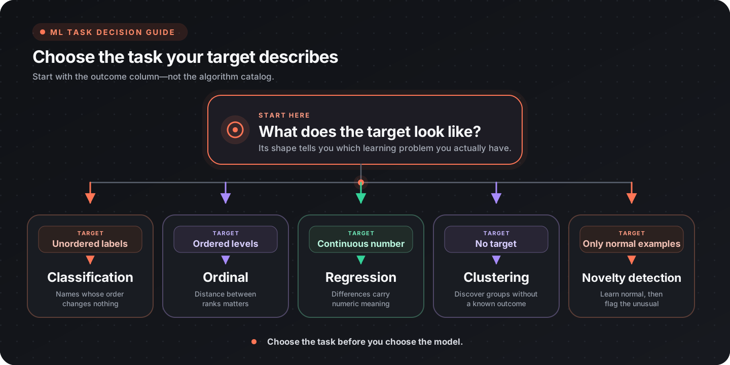
A Flow-Like decision map that routes unordered labels to classification, ordered levels to ordinal learning, continuous numbers to regression, missing targets to clustering, and normal-only examples to novelty detection

The target looks like	Task	Deciding test
Names with no inherent order	Classification	Reordering the labels changes nothing about the problem
Levels with an order	Ordinal	Being off by two levels is worse than being off by one
A continuous number	Regression	The difference between 10 and 12 means the same as between 100 and 102
No target column	Clustering	You want groups, but nothing supplies the correct groups
No target column, and the columns themselves are the problem	Dimensionality reduction	You want fewer, denser columns or a two-dimensional picture, not row groups
Only examples of normal behaviour	Novelty detection with One-Class SVM	New rows should be flagged as inliers or outliers

Ordinal is its own task

A classifier discards the order of the levels, so predicting low when the truth is high costs it exactly as much as predicting medium. A regressor does the opposite and invents distances the levels do not carry — high is not exactly twice medium. If your target is a rating, severity grade, tier, or Likert answer, start in the Ordinal family.

If a five-star review predicted as one star is a worse mistake than one predicted as four, the order carries information and a classifier will throw it away.

Order the target labels

Ordinal trainers need to know which level is lowest. Numeric labels order numerically — integers are parsed before floats, so "1", "2", "10" sorts 1 < 2 < 10, not lexicographically. Non-numeric labels have no inferable order, so training fails rather than guessing: supply the Class Order pin as a comma-separated list, lowest first (low, medium, high). Each trainer reports back the order it actually used, and whether it came from your list or from reading the labels as numbers. Check that output first whenever an ordinal model behaves oddly.

Use a model trained elsewhere

The ONNX inference family runs compatible models that were trained elsewhere and exported to ONNX. Validate the model’s expected tensors and reproduce its preprocessing exactly.

Choose models and transforms

Start with the simplest model that matches the target and constraints. Compare alternatives on the same untouched evaluation set; a more complex model earns its place only when it improves the metric that matters.

Classification

Model	Node	Pick it when	Watch out for
Decision Tree	Train Classifier (Decision Tree)	You need rules a person can read and defend	Unlimited depth memorizes the training set; set Max Depth or Min Samples Leaf
Random Forest	Train Classifier (Random Forest)	You want the strongest tabular baseline with little tuning	Size and fit time grow linearly with ensemble size, and a fixed seed still does not make fits bit-identical across processes
AdaBoost	Train Classifier (AdaBoost)	The signal is weak and one tree underfits	Far more sensitive to label noise and outliers than Random Forest, and equally non-reproducible bit-for-bit
Logistic Regression	Train Classifier (Logistic Regression)	You need calibrated probabilities and readable coefficients	Linear in the features, and the solver needs comparable scales — fit a Feature Scaler first
Gaussian Naive Bayes	Train Classifier (Naive Bayes)	You want a one-pass baseline to beat	Assumes features are independent and roughly normal within each class
Multinomial Naive Bayes	Train Classifier (Multinomial Naive Bayes)	The input is counts or TF-IDF weights from text	Features must be non-negative, so centred or standardized vectors are rejected
SVM	Train Classifier (SVM)	Classes separate along a non-linear boundary in a modest number of rows	One-vs-all training builds a dense n×n kernel matrix per class, so memory grows quadratically with rows
K-Nearest Neighbours	Train Classifier (K-Nearest Neighbours)	The boundary is irregular and the feature count is small	The model embeds a verbatim copy of the training set, so personal data in it travels inside every saved model file
One-Class SVM	Fit Novelty Detection (One-Class SVM)	You have normal rows only and want outliers flagged	It answers inlier or outlier, not which class; Nu bounds the fraction of training rows treated as contaminated

Regression

Model	Node	Pick it when	Watch out for
Linear Regression	Train Regression (Linear)	You want the plainest possible baseline for a continuous target	No regularization at all, so correlated or numerous features give unstable coefficients
Ridge / Lasso / ElasticNet	Train Regressor (Ridge/Lasso/ElasticNet)	There are many features and some are irrelevant	The penalty is scale-dependent, so scale first or the penalty falls unevenly across columns
GLM / Tweedie	Train Regressor (GLM / Tweedie)	The target is counts, positive skewed amounts, or heavy-tailed	The chosen distribution must match the target; a mismatch can diverge to non-finite coefficients
SVM regression	Train Regressor (SVM)	The target bends non-linearly with the features	The solver builds a dense n×n kernel matrix, and there are no coefficients to interpret
K-Nearest Neighbours	Train Regressor (K-Nearest Neighbours)	Local averaging beats a global formula	The model carries the whole training set, and averaging neighbours cannot predict outside the observed target range

Ordinal

Model	Node	Pick it when	Watch out for
Proportional Odds	Train Ordinal Model (Proportional Odds)	Default first choice; you want calibrated per-level probabilities and one readable coefficient vector	One shared coefficient vector across all cut points is the default assumption — Free Features frees chosen features into one slope per cut point, at the price of a non-zero Crossing Rate — and the gradient fit needs scaled features
Ordinal Ridge	Train Ordinal Model (Ridge)	You want a fast closed-form baseline with many levels or many features	It returns the level and its latent score, but no calibrated probabilities
Frank & Hall	Train Ordinal Model (Frank & Hall)	The boundary between levels bends and you want a non-linear base learner on an ordered target: Decision Tree, Random Forest, or Gaussian Naive Bayes when rows are few relative to columns	It predicts by counting how many of the K−1 cut models say yes, so there are no calibrated probabilities and no coefficient vector
Continuation Ratio	Train Ordinal Model (Continuation Ratio)	The levels are a sequential process that can halt: escalation tiers, disease stages, funnel depth	Stricter than the others — every declared level must occur, middle ones included — and higher levels are fitted on fewer rows
Adjacent Category	Train Ordinal Model (Adjacent Category)	The question is about one step up: ratings, severity grades, Likert answers	Its coefficients mean “level k+1 versus level k”, not “at or below cut k”, and the bottom-to-top effect is (K−1) times the per-step effect
Neural CORAL/CORN	Train Ordinal Model (Neural CORAL/CORN)	The level is genuinely not monotone in the features and you still need probabilities	With no hidden layers CORAL is exactly Proportional Odds with Loss = AllThreshold and Margin = Logistic, and CORN is exactly Continuation Ratio with the logit link, so prefer those for linear problems

The neural node is the only ordinal trainer that is non-linear, probabilistic, and rank-consistent at once. That combination costs a non-convex objective — the seed changes the fit — and far more rows than a linear model. Read its Architecture output, which reports parameter count next to row count, before trusting a training score.

Clustering

Model	Node	Pick it when	Watch out for
KMeans	Train Clustering (KMeans)	The groups are compact and you can name a cluster count	You must choose k up front, and the distance metric makes unscaled columns dominate
DBSCAN	Train Clustering (DBSCAN)	The groups have irregular shapes and you want noise identified	It reports clusters and noise counts for the rows it was given and returns no reusable model handle
Gaussian Mixture	Fit Clustering (Gaussian Mixture)	You want soft membership and per-component covariance	linfa hard-codes its internal RNG at seed 42, so the Seed pin only re-orders rows; a tiny mixture weight means that component captured almost nothing

Clusters do not acquire business meaning automatically. Review representative records and check stability across seeds and samples before attaching labels to them.

Dimensionality reduction

Method	Node	Pick it when	Watch out for
PCA	PCA Reduction	Correlated numeric columns should be compressed while keeping linear variance	Linear only; it writes reduced vectors back into the table and returns explained variance, not a reusable fitted model
t-SNE	t-SNE Reduction	You want a two- or three-dimensional picture for exploration	Transductive, so it produces no reusable model, and distances and cluster sizes in the layout carry no validated meaning

Preprocessing

Step	Node	Pick it when	Watch out for
Feature Scaler	Fit Feature Scaler	Any distance- or gradient-based model is downstream: Logistic Regression, Elastic Net, SVM, KNN, Gaussian Mixture, and every ordinal trainer except Frank & Hall, whose base learners need no scaling	It learns offsets and scales from the data it sees, so fit it on the training split only
TF-IDF Vectorizer	Fit TF-IDF Vectorizer	A text column has to become numeric vectors for a classifier	linfa recomputes the inverse document frequencies from the corpus being transformed, so vectors are only comparable within a single Apply Transform run
Apply Transform	Apply Transform	A fitted transformer has to be replayed on another table	Pass the same fitted model you trained with; a second Fit call produces different statistics

Build a leakage-safe pipeline

The sequence matters. Split before fitting anything that learns from data, then carry those fitted transforms forward as part of the model contract.

Stage	Node	Why it is in this order
Split	Split Dataset, Stratified Split	Split before anything looks at the data; stratify when class proportions are uneven
Fit scaling on train	Fit Feature Scaler	Learns offsets and scales without looking at the test split
Apply the scaler to every split	Apply Transform	Replays the exact offsets and scales learned on train
Train	Any trainer from the tables above	One model, one documented configuration
Evaluate	Accuracy, Ordinal Metrics, Regression Metrics	On the untouched split, with a task-appropriate metric
Save	Save Model	Save the predictor and each fitted transformer separately, then version them as one contract
Predict	Predict	Same feature order, types, and transforms as training

A transform that learns from data is itself a fitted model. That is the whole point of Feature Scaler being a fitted model rather than a formula: you fit it once on the training split and pass that same fitted object to Apply Transform for validation, test, and inference. Fitting a second scaler on the test split gives that split its own statistics and quietly invalidates the comparison.

Supporting dataset nodes: K-Fold Split runs its connected branch once per fold, Shuffle Dataset and Sample Dataset reorder or subset rows. For time-dependent data, split chronologically instead of randomizing future observations into the training set.

Let the catalog compare candidates

Auto Classifier cross-validates several classifier families and retrains the winner; Auto Ordinal does the same for ordered targets and ranks by a distance-aware metric. Feed the reported best model type into Grid Search or Ordinal Grid Search to tune it, including an OrdinalNeural winner — its grid takes hidden_layers, head, activation, alpha, learning_rate and max_iterations, but keep it small, because every combination trains a network from scratch on every fold. Use the ordinal pair for ordered targets — Auto Classifier resolves the target without its order and ranks by accuracy or macro F1, either of which scores a five-level miss exactly like a one-level one. See Auto Training.

Evaluate on untouched data

Task	Nodes	Note
Classification	Accuracy, Confusion Matrix	Accuracy alone hides poor minority-class performance; read the matrix
Binary classification with probabilities	ROC-AUC & Log Loss	Needs a P(positive class) column, which batch prediction does not produce — see below
Regression	Regression Metrics	MSE, RMSE, MAE, and R²; also check residual patterns, not one aggregate
Ordinal	Ordinal Metrics	Quadratic weighted kappa as headline, plus linear kappa, macro error, and rank correlation
Clustering	Silhouette Score	Distances are euclidean, so scale features before reading the score

Accuracy is the wrong headline for an ordered target because it gives no partial credit for a near miss: one level off counts exactly like four levels off. Ordinal Metrics weights every miss by how far off it was.

ROC-AUC needs a column of P(positive class), and Predict does not write one. In Database mode it writes the predicted class only; the confidence figure exists solely on the struct returned by its Vector mode, one row at a time. So building that column means looping rows through Vector-mode Predict and writing the value yourself.

Converting it correctly matters as much as producing it: confidence is the winning class’s probability, not the positive class’s. Use it directly where the prediction is the positive class and 1 - confidence elsewhere. A raw confidence column produces a meaningless curve and does not error.

Only models that carry a probability model report a confidence at all. Decision Tree, Random Forest, AdaBoost, both Naive Bayes variants, Frank & Hall, Ordinal Ridge and every regressor return none, so ROC-AUC and log loss are unavailable for them.

To inspect a fitted model: Model Info for general metadata, Get Coefficients for linear regression, Get Centroids for KMeans, and Feature Importance for Decision Tree, Random Forest, and AdaBoost.

Ship the training contract

Need	Node
Save through the path abstraction	Save Model
Load through the path abstraction	Load Model
Save as raw binary (Fory format)	Save Model (Binary)
Load raw binary (Fory format)	Load Model (Binary)
Run a model on prepared features	Predict

Each Save Model call accepts one model handle. Persist the predictor and every fitted transformer with separate save nodes or paths, then give the set one shared version in your model card or deployment metadata.

Inference has to reproduce the training feature order, types, missing-value handling, and every fitted transform. Validate the input schema before calling Predict, and store a short model card with the artifact: training data version, feature schema, target definition, metrics, intended use, limitations, and owner.

For KNN models, remember that the artifact contains the training rows themselves. Apply the same access controls to the model file that you apply to the source table.